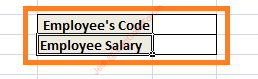
Step 2) Click on the cell where you want to apply the VLOOKUP function. In this case, it would be cell alongside Employee’s Salary with cell reference ‘F3’.
Step 3) Argument 1: Enter the cell reference which contains the value to be searched in the lookup table. In this case, ‘F2’ is the reference index which will contain Employee’s Code to match for corresponding Employee’s Salary in the lookup table.
Step 4) Argument 2: In the second argument, we enter the lookup table or the table array. However, in this instance, we have the lookup table situated in another sheet in the same workbook. Therefore, for building a relationship we need to enter address of the lookup table as Sheet2!A2:B25 – (A2:B25 refers to the lookup table in sheet 2)
Step 6) Argument 4: Last Argument refers to the Exact Matches (FALSE) or Approximate Matches (TRUE). In this instance, we want to retrieve the exact matches for the Employee’s Salary.
Step 7) Press Enter and when you enter the Employee’s Code in the cell, you will be returned with corresponding Employee’s Salary for that Employee’s Code.
The above 3 scenarios explain the working of VLOOKUP Functions. You can play around using more instances. VLOOKUP is an important feature present in MS-Excel which allows you to manage data more efficiently.